The Case of a Fixed Strategy Outcome
When building a long-term stock trading portfolio we should have a different set of considerations compared to managing a traditional long-term investment portfolio. At the center of it all, we will have to tackle the average length of the trading interval and what we might be able to extract from it.
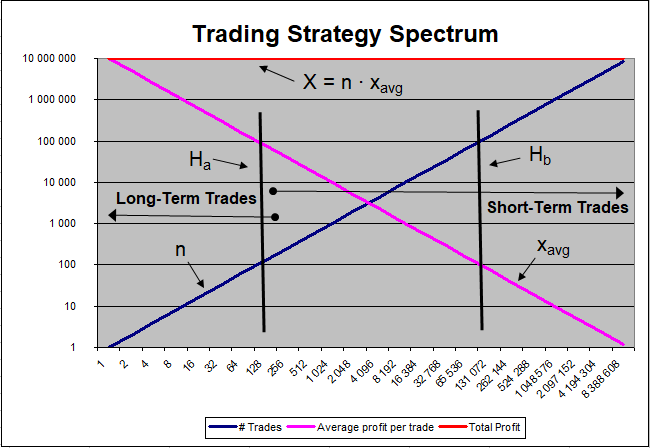
Both types of strategies will respond to the same set of equations as presented in Portfolio Building. The big difference is they reside at either end of the trading spectrum. This was illustrated with a chart in Portfolio Building. Here is the same chart with some added details:
The above chart still responds to the payoff matrix equation and its equivalents: $$F(t) = F_0 + X = F_0 + \Sigma x_i = F_0 + \Sigma_i^n (H \cdot \Delta P) = F_0 + n \cdot \bar x$$ It shows a constant total profit of $X = n \cdot \bar x$ where $\bar x$ is the average net profit per trade, and $n$ the number of executed trades over the life of the portfolio. The greater the number of trades, the lower the average net profit per trade, and, on average, the smaller the trading interval. Any strategy subset achieving $X$ is admissible since all those strategies would give the same answer. This is reducing the whole trading portfolio to very simple variables, just two numbers: $X = n \cdot \bar x$. One of which, $n$, is just the counter: $n = n_{-1} + 1$.
The chart separates short-term trading portfolios and long-term investment portfolios. It is a fuzzy and arbitrary definition (separation is at about 250 trades), it could be at 1,000 trades should it better fit your own vision of what constitutes a trading portfolio. Short-term trading portfolios tend to have a large number of trades with a small average net profit per trade $\bar x$ while long-term investment portfolios have a low number of trades with a much larger $\bar x$. Both can achieve the same results as shown with strategies $H_a$ and $H_b$. All possible combination in this trading spectrum is available and will give the same $X$ result, not just at strategy $H_a$ or $H_b$. We can achieve the same result doing 100 trades or 100,000 trades, the difference will only be in $\bar x$, our average net profit per trade.
If strategy $H_a$ gives the same result as strategy $H_b$, does it matter which one we use since we would end up with the same amount in our trading accounts? Choosing one would more depend on our trading preferences or which of the two programs we were able to find or design since these two strategies would not behave the same; nor could they have the exact same code. You modify the trading script, and transform $H_a$ into $H_b$, would you have gained anything?
Something else the above chart is saying; there are a multitude of trading strategies that can generate the same amount of profits as illustrated by: $X = \$10,000,000$. To improve on the outcome, you have to increase $X$. Either by increasing $n$, $\bar x$, or both. The chart shows the x-axis as a power of two ($2^n$). In the chart, each time you double the number of trades, $\bar x$ is divided by 2 to maintain $X$.
A different look at the above chart (at normal scale) tells another story even if the data is exactly the same.

The total profit $X$ generated by the trading strategy was broken down into its most basic elements $n$ and $\bar x$. It did not matter how you traded and under which conditions. In the end, all that counted were those two numbers and what they left in the trading account. The payoff matrix was totally trade agnostic: $X = \Sigma_i^n (H \cdot \Delta P) = n \cdot \bar x$. You could use whatever you had at your disposal as long as it generated a positive payoff: $n \cdot \bar x > 0$. In all scenarios, the number of trades can only be positive $n > 0$ making $\bar x$ (the strategy's edge) responsible for positive or negative results. Note that $n = 0$ is a trivial case since there would be absolutely no generated profits due to no trades being executed ($0 \cdot \bar x = 0$) whatever the type of portfolio you might consider.
No matter what the trading strategy might be, the above chart's general appearance would be the same, it is only the scale that would change, meaning $X$. Increasing either $n$ and/or $\bar x$ will improve overall performance. Therefore, this would tend to change the nature of the game. It becomes a game of averages with actually a single goal which is increasing $\bar x$ as much as possible over the largest number of trades possible.
In the above chart $X_a = X_b = \$10,000,000$. If you increased $n$ in $X_a$ by a factor of 10 you would get $X_c = 100,000 \cdot \$1,000 = \$100,000,000$, achieved simply by increasing the number of trades (see *Portfolio Building* for $X_a$ and $X_b$). But, you cannot increase $n$ just like that without appropriate changes to the trading strategy itself.
The question should then become: how could we increase the number of trades while keeping the average net profit per trade stable? The problem has no "sentiments", no psychological influences, no moon phase. It is just a practical question. How do you increase the number of trades without sacrificing too much of $\bar x$ in the process?
The problem is not easy to solve. All the equations presented assumed full market exposure, therefore, where would the money come from? One way could be to find shorter trading intervals with about the same profit potential?
I discused the portfolio rebalancing problem in a previous article. It provided the following equation for a rebalancing portfolio: $$F(t) = F_0 + n \cdot \bar x = F_0 + y \cdot rb \cdot j \cdot E[tr] \cdot b(t) \cdot E[PT]$$ where $n$ was again the number of trades, $y$ the number of years the strategy was applied, $rb$ the number of rebalancing per year, $j$ the number of stocks in the portfolio, $E[tr]$ the expected turnover rate, $b(t)$ the betting function, and $E[PT]$ the expected profit target or the expected average percent profit on the average trade. With this equation, we could make estimates on the outcome of a trading strategy since $n \to y \cdot rb \cdot j \cdot E[tr]$, and $\bar x \to b(t) \cdot E[PT]$. Due to the law of large numbers, we would also have that $E[tr] \to \overline {tr}$ where the turnover rate approaches a constant, and $E[PT] \to \bar g_w$ the average gain percent per trade.
If you rebalanced 100 stocks on a weekly basis for 15 years with a monthly turnover rate of 60% you would get for estimate: $15 \cdot 52 \cdot 100 \cdot \frac{0.60}{4} = 11,700$ trades. Those trades were not executed because of some fundamental data, some technical indicator or sentiment measure. They were executed simply because rebalancing was requested on a weekly basis on those 100 stocks. A strategy design or an administrative decision that would effectively impact almost all the trades over the life of the portfolio.
This made the self.Schedule.On() command line responsible for the trades. And not some kind of indicator (fundamental or technical) used in the program code.
It is not the trading signal that is generating the trades, it's simply the scheduled rebalancing. In a 100 stock scenario, the weight of each stock is 0.01. If all stocks go up by 5%, they still all have the same weight (0.01). It is the disequilibrium from the average price movement that will trigger trades. However, if you follow the rules of rebalancing, losses are not necessarily immediately acknowledged. To make the problem easy, make half the portfolio go up and the other half go down. The rebalancing will sell part of the shares held that went up generating a profit for each one of them. However, for the shares that went down, the loss is not taken, shares are not sold. Instead, new shares are bought to reset the weight to 0.01. Therefore, only upward-moving stocks are sold generating profits. In a way, the rebalancing is selling on the way up and buying the dips or on the way down.
So, 50 stocks recorded partial sales with profits, and the other 50 saw their holdings increased without registering a loss. Evidently, this directly affects the strategy's overall hit rate.
The how you set the rescheduling gets to be important just as the number of stocks on which this rebalancing will be done. If you did the above with only 10 stocks, you would get: $15 \cdot 52 \cdot 10 \cdot 0.15 = 1,170$ trades, as should be expected, 10 times fewer trades. But this also implies that we would now have 0.10 as the weight for each stock making the bet size 10 times larger.
If you rescheduled on a daily basis for the 100 stock scenario, you would get: $15 \cdot 252 \cdot 100 \cdot 0.03 \approx 11,340$ trades. Not because your trading signal was forcing the execution of trades, but simply due to the rebalancing itself. Each day, stocks that rosed in price above their 0.01 weight would see some of their shares being sold pushing money back into the trading account.
We can see the expected turnover rate is playing a major role in this estimation. It is a number we can get from the first simulation we do based on the rebalancing period.
All that counted for the rebalancing was the rise in price above the average price movement of the stocks in the portfolio. It did not ask for any other reasons, predictive or not. The question of why the price rose was not even a question. It simply executed a partial sale of some of the shares in its rising stocks in order to return each of the stock weights to 0.01. The trade triggering signal was not even involved in the process, except maybe coincidentally. However, the daily variance was. It simply did not matter how or why the price moved. The weight going above 0.01 was the main criterion for the partial sale, even if it might have appeared at the same time as some other trade triggering mechanism.
There was no feedback from the trading procedures that the trade triggering mechanism was carrying the day. Even if the price movement could be explained as some quasi-random phenomena, the trades would still be executed for the simple reason that the price moved. And for a trading strategy, this would tend to change the nature of the game.
If just two numbers resume all of a portfolio's trading activity over its entire lifespan, shouldn't we concentrate all our efforts and trading procedures to increasing those two numbers as much as we can with all the tools we have?
© 2021, Guy Fleury